Hi blog!

So I’ve returned to work after a 3.5 week vacation to Bali! Woo! Time to catch up on some long non-blogging. But before that...

Here’s where my crazy Uncle Jimmy took me and the missus for a few days… Gili Gede (meaning “Little Island Big”) off the coast of Lombok (which appears to be experiencing a gold-rush, so go now before its all built up!).
The ferry between Bali and Lombok took us across the legendary "Wallace Line", though my total ignorance of systematics means I couldn't really tell the difference in flora and fauna between the islands. (Though we did see a HUGE monitor lizard near a brick-making operation.)

I stayed out at the end of this pier on the lower left at the “Secret Island Resort”. (Note the vessel that took us snorkeling to the immediate South... the "Scorpio".
And here's an actual shot of the infamous "Rocky Docky" with the lovely Heather in the foreground:
The reef was right over the edge of the pier, so snorkeling to see all the corals and fishies was optional. You could just look over the edge! Excellent!

Anyways, I've been getting my head back into things and am writing a few blog posts about what’s going on in my world-of-science. So expect a deluge of catch-up posts during the next day or two… (continued...)

Manuscript plans?

So I’m a bit over one year into my postdoc. What have I got to show for myself? Well, plenty of work, but not any papers, or even written manuscripts, so that’s a bit of a problem. Can I turn my first set of genome sequencing data into a manuscript?

Seems likely. I collected >5 Gigabases of Illumina sequence data from several Haemophilus influenzae chromosomes, and this could be used as the basis of a manuscript. I obtained data from a donor strain (86-028NP NovR NalR) and a recipient strain (Rd, RR722) as control data (in order to evaluate the ability of the sequencing and read alignment to correctly identify polymorphisms). I also obtained data from two individual transformants and a pool of four transformants to identify donor alleles in transformed recipient chromosomes. I even found some things out.

Does this a paper make? One outstanding issue is that, in spite of being a lot of data, which has required a fair amount of work to get a handle on, there is not a tremendous amount of biologically relevant data. Yes, I obtained extremely accurate and comprehensive data for the four transformants sequenced. But it was still only four transformants. There are some biologically meaningful results; they just aren’t terribly novel or statistically robust. The bigger biologically meaningful results will have to wait until we can collect more data.

So to turn this into something publishable, the approach and method need to be important enough (and made explicit enough) to be of value to others. So far, I have not done anything in my analysis that is truly novel, but I have managed to produce the bare-bones of a “pipeline” for measuring allele frequencies from pools, and identifying recombination tracts in transformants. The data we got was also extremely high coverage, so we were able to see the limits of the technology fairly well: i.e. depth-of-coverage variation, errors, and issues with read alignment.

Though everything I’ve done so far uses “off-the-shelf” bioinformatics tools, there are so many people trying to do similar things, it might be useful to write a paper that is sort of an “application” of the technology and tools I’ve been using. It took me months to piece everything together, so maybe I could save someone else some time by having everything in one place. But with each passing day, the value of such a paper is probably diminishing, so I’d best get started!

There are still a few analyses I’d like to do that would give the paper a little more spice:

1. Structural variant analysis: This is something that will involve our collaborators at UVA, who are experts. We can see these pretty well (at least the larger ones), but something systematic has yet to be done.
2. Reciprocal read mapping: I’ve mapped all the data to both the donor and recipient genomes, but I have not really fully leveraged this fact. The read alignment artifacts that arise mapping data from one strain onto the other could be handled much better, if I was able to assign individual reads to either of the two reference genomes, based on the mapping quality. I’d really like to do this. It’d be novel, mainly because most people sequencing are doing SNP discovery. I already have all my SNPs discovered, so doing an extra good job at calling SNP frequencies using reciprocal alignment would be at least something new. This will take a bit of work, however, and I’ll need to figure out the best computational way to do it. Aside from doing uber-detailed error analysis for a technical paper, I think this is really the best chance to make a novel contribution bioinformatically.

Here is a rough outline of the manuscript, as I’m viewing it so far:

1. Introduction

• Many bacteria become naturally competent. Natural transformation is important in evolution.
• Previous sequencing studies have focused on only a handful of defined constructs. (Bacillus, Helicobacter, Actinobacillus).
• For any organism, the total extent of recombined fragments in individual transformants has never been directly evaluated, and the factors dictating the chance of transformation are only poorly understood as a result.
• Haemophilus influenzae is a model system for natural transformation. The mechanism is well-defined. Transformation is efficient in the lab strain.
• The extensive natural genetic variation between H. influenzae strains provides tens of thousands of markers to identify recombination tracts in individual transformants. Not only single-nucleotide, but structural variation in the form of indels and other rearrangments. The “supragenome” hypothesis.
• We investigated the use of massively parallel sequencing (or “next generation sequencing”, NGS) to characterize natural transformation at a whole-genome scale.
• Our results show the Illumina platform to be an excellent method to obtain nearly exhaustive information on recombination tracts in individual transformants. Our approach uses the alignment of sequence reads to both donor and recipient reference sequences. We obtained donor and recipient genome sequence as controls for evaluating sequencing error, depth of coverage, and polymorphism identification. We also obtained the sequence data from two individual transformants and a pool of four transformants.
• Individual recombination tracts are longer than previously appreciated and can bring hundreds of polymorphisms from donor to recipient chromosomes (both single-nucleotide, insertion, deletion, and insertional deletion). However, recombination tracts often appear interrupted by or terminated at sites of structural variation between the two genomes. This shows that such variation are barriers to strand exchange and/or are preferred mismatch repair substrates.

2. Materials and Methods

• Strains
• DNA
• Transformations
• Library preparation
• Illumina sequencing and initial data processing pipeline
• Reference genome alignment by MUMmer, MAUVE
• Reciprocal read alignment by BWA
• SAMtools pileup
• Galaxy pileup parser
• Variant frequency analysis
• Assignment of reads (unimplemented)
• Donor segment calling
• Analysis of structural variation by HYDRA

3. Results

• Genetic transformation of competent cells: Marker to marker variation. Dependence on sequence identity. Congression and linkage
  
• Illumina sequencing and read alignment: Table of sequencing results and fraction of mapped reads. Variation in depth-of-coverage. Sources of sequencing error and read mapping artifacts. Reciprocal read alignment? Varying alignment stringency?
  
• Comparison of donor and recipient strains. Identification of SNPs and structural variants between the donor and recipient strains. Comparison to whole-genome alignment methods.
• Identification of donor alleles in transformed recipient chromosomes. Accounting for SV alleles. Identifying novel alleles.
• Identification of allele frequencies in a pool of four transformants.
• Identification of donor segments and putative recombination tracts
• Enrichment of SVs at donor segment breakpoints

4. Discussion

• A first look at transformation… still few transformants
• Excellent method. Limitations are circumvented by very high coverage, knowledge of both donor and recipient genome sequences, and the use of reciprocal read alignment (unimplemented)
• Big recombination tracts. Evidence of mismatch repair. SVs as blocks to recombination tract progression.
• Speculations: Hotspots? Role of uptake specificity? Supragenome transfer?
• Future: Aside from collecting more transformants, making a transformation frequency map to investigate the “cis-acting” factors controlling the efficiency of transformation. Long-term utility in understanding the population genetics of human pathogens.

Still a rough outline, but something to start with.... (continued...)

Degenerate Uptake: Pilot Study

Something to blog about! (Wow; it's been over a month... sorry to my three loyal blog readers.)

I’ve gotten around to doing a pilot-scale experiment on the specificity of H. influenzae DNA uptake for the “uptake signal sequence” (USS). The USS is a ~29 base pair motif highly abundant in the H. influenzae genome, and sites that match the consensus USS are known to be preferred substrates for DNA uptake by competent cells. The presence of many USS in the chromosome is presumed to be why H. influenzae competent cells prefer H. influenzae DNA over DNA from other organisms.

However, little is known about how the structure of USS contributes to uptake of USS-containing fragments: Limited analyses of mutations of a DNA fragment containing a consensus USS suggests that some but not all informative positions in the USS motif are important to uptake, indicating that other forces (perhaps later steps in transformation) contribute to the structure of the USS motif.

To carefully dissect uptake specificity for the USS motif, we have devised an enrichment experiment:
(1) A complex pool of DNA fragments containing a degenerate USS library is incubated with competent cells.
(2) The fragments preferentially taken up by cells are purified from the periplasm.
(3) DNA sequencing is used to compare the input and periplasm-purified pools of sequences.

Details and Pilot-scale Results:


I’ve previously discussed the design of the input DNA pools. The control 200 bp construct is designed to already contain the sequences needed for Illumina single-end sequencing, along with a 32 bp consensus USS site near the middle of the fragment. The test construct is the same, except the USS is degenerate, having a 24% chance of a non-consensus base at each position. Thus in the degenerate-USS pool, the average site has ~7-8 mismatches from the consensus sequence.

The expectation is that, while the consensus-USS construct (USS-C) will be taken up by cells well, the degenerate-USS construct (USS-D) will be taken up more poorly, since it contains many suboptimal sequences (i.e. it is less uniformly delicious). Indeed this is the case, with USS-C being taken up about 10 times better than USS-D at sub-saturating DNA concentrations (see below). The notion is that comparing the USS-D input to that taken up by cells will provide a precise measurement of uptake specificity for the USS (i.e. which sequences are tastiest). We think this will tell us a lot about the mechanism of uptake.

It occurred to me a couple weeks ago that before moving on to the data collection (i.e. the DNA sequencing), I should first make sure that the USS-D fragments recovered from the periplasmic purification are taken up better than the original USS-D input (i.e. the competent cells selected more delicious sequences). This would provide the clearest indication that the experiment worked and the material is worth sequencing. It is!

I compared the uptake of USS-C and USS-D before and after periplasmic purification of taken up DNA from rec-2 competent cells across a range of DNA concentrations. Here are the results:
A and B show the % DNA uptake for USS-C and USS-D, respectively, for different amounts of added DNA (to 200 ml competent cultures). C and D show the same data: C is a dose-response curve, and D is a double-reciprocal plot (since I used 2 ng of hot label, along with an additional amount of cold label for these experiments).

Input USS-C and periplasm-purified USS-C were quite similar, while periplasm-purified USS-D was taken up substantially better than input USS-D.

Notably, at low (sub-saturating) concentrations of DNA, periplasm-purified USS-D is taken up less well than USS-C, while at high (saturating) concentrations similar amounts of DNA are taken up. Also of note is that the input USS-D does not saturate until higher concentrations than the other three samples.

This is all good news. I left out a fair number of details, but this pilot-scale experiments is extremely encouraging. Next week, I plan to repeat the experiment, but this time on an appropriate scale for recovering samples for sequencing. I will also investigate how periplasm-purified USS-D samples behave when recovered from uptake experiments with varying amounts of DNA. I expect that at sub-saturating concentration, the cells will be less “picky”, such that periplasm-purified USS-D will be taken up less well than that purified from saturating concentration. This would provide a useful experimental condition, as in the sequence analysis we would be able to investigate the role of competition in shaping USS specificity.

I think this might end up working swimmingly... Onward! (continued...)

Mining some old array data

So in an effort to re-examine some of the lab’s old array data, I made a fairly simple R script to plot the change in expression of competence genes, putative purR-regulated genes, and genes involved in utilizing secondary sugars. We no longer have our expensive license for fancy-pants software, but all I needed to do was some arithematic to columns, and then find the rows of interest, so it’s R-tastic!

I looked at a time course dataset, in which expression was monitored over the course of growth in sBHI and after transfer to MIV. I also looked at a single one-off array comparing purR- to purR+ strains growing in late-log +cAMP.

Here’s the results for the time course. All values are normalized to the first time point. Blue are sBHI timepoints, and red are MIV timepoints. MIV cultures were split from the sBHI cultures at t=0 minutes.

It’s pretty clear that the competence genes are strongly induced in MIV, but are also induced in late-log phase, as expected. Putative PurR-regulated genes are strongly and quickly induced in MIV, indicating that purine pools are quickly depleted, and the purine biosynthetic pathway is activated quite quickly (much faster than the competence genes, it appears). The “non-PTS” genes (several genes induced by CRP when cAMP levels are high) appear to be briefly weakly induced in MIV, as well as being weakly induced in late-log.

Here’s the same sets of genes plotted as the ratio of expression in purR- vs purR+ cultures (late-log, induced with cAMP). Here, I plot the ratios from both array elements for each gene (open and closed circles) and colored them just so they’d be easy to see. Also note, I normalized everything to the median ratio to account for dye effects (under the assumption that the median gene is not PurR regulated). Again, strong induction of the putative purine-regulated genes, a weak repression of the competence genes (presumably due to purine repression), and not much happening with the non-PTS sugars.


Conclusion: Nothing we didn’t already suspect, but it’s good to see that things are behaved as expected. One point of note is that the hypothesized regulation of rec2 by PurR isn’t something that jumps out of this, but if purine repression acts upstream of rec2, we wouldn’t be able to see the effects of deleting PurR here anyways… (continued...)

SNP densities

So I’ve been writing yet another grant, which has been distracting me from blogging (this isn't supposed to be a monthly blog, but this will hopefully be the last grant application for a while).

But I’ve also been doing several analyses lately. Here’s one. I took the sequences of an ~300 kb restriction fragment from three H. influenzae isolates (Rd, 86-028NP, and PittGG). They’re all similarly divergent from each other (~2.5%), and I wondered how well the level of divergence of Rd vs NP and Rd vs GG correlated along the chromosome...

So I aligned the sequences in Mauve, took its SNP calling output, and did a couple simple sliding window analyses inside R (using the zoo package for rolling means). Here’s what divergence looked like averaged over 5 kb windows (click to enlarge):
The divergence between Rd and the two other isolates are quite well correlated (r2= 0.8, using linear modeling). But since NP and GG are similarly divergent, I made two other plots.

First, here’s a comparison of the density of SNPs that are shared by NP and GG and those that are unique to either NP or GG:
The correlation is a lot worse (r2=0.4).

And if I further break the “unshared” line into NP and GG-specific SNPs (i.e. positions are different between Rd and NP but not GG, and vice versa).
The correlation is worse still (r2=0.2)

Similar results applied to smaller windows, but the plots looked a lot messier. Note that it’s not exactly totally straightforward to measure SNP density... What does one do at indels?? I just ignored them, so the results above are rough. Part of the reason I focused on only a co-linear segment of chromosome was to minimize this problem, but there are still several indels between each of the three strains.

Indels aside, what’s this mean? One of the goals of my transformation frequency mapping is to be able to distinguish the effects of sequence divergence on transformation from the effects of other local chromosomal properties (base composition, sequence motifs, etc.). Since NP and GG have correlated SNP densities relative to Rd, transformation frequencies across the Rd chromosome are expected to also be correlated. Discrepencies in transformation frequency by NP and GG donors could indicate that SNPs specific to the isolates are somehow modulating transformation independent of divergence per se.

Distinguishing chromosome “position effects” from sequence divergence will probably require a third donor DNA. Deciding what this would be requires some thought. All of the sequence H. influenzae are similarly divergent from Rd (and for the most part each other), and phylogeny poorly distinguishes separate clades (i.e. they kind of give a star phylogeny).

So I should use either a strain much more closely related to Rd or one more distantly related (perhaps another species). Using a closely related strain has the advantage that transformation frequencies are expected to be higher and divergence will play less of a role, making the focus more on divergence-independent factors, but I would also have far fewer markers.

Based on MLST comparisons, several strains are sisters of Rd (RM7033, RM7429, RM7271). These assignments are made in several phylogenetic and put the three at ~0.5% divergent from Rd. So I would expect that RM7033 (for example) would have ~6000 SNPs from Rd (far more than our Rd or the other sequenced Rd), ample to have markers across the chromosome... (continued...)

Chromosome "Position Effect"

I got some data for the transformation frequency at five different markers. They varied. This isn’t anything ground-breaking; reports of a "position effect" for transformation go back decades and a couple of recent studies in other organisms bear it out. The underlying cause of variation in transformation rate at different positions likely stem from two sources: the physical structure of the chromosome and the sequence composition of the recombination substrates. The former case is reasonably well-worked out for analogous processes in eukaryotes: For example, in yeast, heterochromatic regions are recalcitrant to recombination, but these sites become recombinogenic in mutants with defective heterochromatin assembly. Sequence composition has also been shown to affect the efficiency of recombinational strand exchange in several different contexts, both genetic and biochemical. This latter type of variation is not traditionally considered a "position effect", but is difficult to distinguish from the former.

Anyways, I wanted preliminary data showing that I can, in fact, detect differences in transformation at different genomic positions, since a big part of my proposed work will involve measuring to very high resolution this position effect...

I used MAP7 donor DNA to transform three independent Rd competent cell preps. MAP7 is highly similar to Rd, except that it carries several point mutations that confer antibiotic resistance. There are likely other unselected differences between Rd and MAP7, but few. Thus, differences between marker transformation rates are likely to predominantly reflect chromosome position effects, rather than sequence divergence between donor and recipient.

This latter point isn’t strictly true: in order to see transformation, a genetic change has to be made, and the selected MAP7 point mutations are genetic differences. But because in our preliminary sequencing data, we saw long stretches of donor-specific DNA with dozens to hundreds of SNPs, I don’t think these single-nucleotide differences are contributing too hugely to the observed variation in transformation rate.

Here’s the data for the five markers individually. Vertical bars indicate the mean transformation frequency per viable cell to the indicated antibiotic resistance allele. The inset circle shows a rough map of the location of the MAP7 markers. (Sorry about the lack of an origin.)
Indeed, I see a ~5-fold range of transformation frequencies, from ~1/500 to ~1/100. Since this is only an arbitrary sampling of five sites, the range of variation across the chromosome could be much higher.

As previously discussed, these values underestimate the transformation frequency per competent cell. Competent cultures typically have both competent and non-competent cells, and the “fraction competence” is typically measured by looking at co-transformation frequencies. These are often higher than expected, even for unlinked markers, a phenomenon termed “congression” and interpreted as a binary distinction between competent and non-competent cells in the culture.

The technical value of this is that I can elevate the observed transformation frequency at one locus by selecting for transformation at another unlinked locus, since this eliminates all non-competent cells from the culture, providing potentially higher sensitivity on our proposed sequencing experiments. It also dampens differences in culture-to-culture variation caused by big differences in fraction competence (not shown).

However, there is at least one old report using Bacillus that suggests congression does not simply reflect a binary distinction between competent and non-competent cells . If cells only came in those two flavors, we would predict that any pair of unlinked markers would show the same level of congression, yet they report that different pairs of markers had different congression frequencies (aside from due to linkage). They go on to suggest an interesting model for their observations, but my concern is more technical:

Does selecting for transformation at different loci affect the tranformation rate at a second unlinked locus?

If the answer is yes, then selection for transformants at a locus would be a poor way to elevate the transformation rate at other unlinked loci, since it would be biased in an unknown way. I also measured co-transformation of Nal resistance and each of the other four. Nal is “unlinked” from all the others (i.e. DNA fragments from standard DNA preps will always be too short to contain the NalR allele with another antibiotic resistance allele), so I can measure “congression” four times.

Here is the data. So, for example, the first bar was calculated as: f(kanR nalR) / f(kanR). This normalizes each bar to the nalR rate (i.e. “the frequency of nalR among kanR transformants”).
The first thing to note is that the scale bar has changed relative to the transformation/cfu. For each of the 3 cultures, there was ~3.5 fold increase in the observed transformation rate, which would be expected if ~1/3 of cells in each culture were competent.

The second thing to note is that selecting for any of the four markers had no effect on the NalR transformation frequency. So the answer to the above question is no. Phew! The Bacillus result was cool, but I’m glad it isn’t the case here. A binary competent/non-competent model is perfectly reasonable in our system (though this does not exclude the possibility of variation among competent cells). With this in hand, I can now plot the co-transformation data with respect to NalR. If selecting for NalR only eliminates non-competent cells but does not change the underlying transformation frequencies per competent cell at the other unlinked markers, then life is good.

Here’s the data. So for example, the first bar was calculated as f(kanR nalR) / f(nalR). This normalizes each bar to its own rate (i.e. “the frequency of kanR among nalR transformants”). For the nalR/competent cells, I used the average of all 12 points in the previous plot.
This data closely resembles that of the first figure, except all the values are ~3.5 -fold higher.

Woo! Next I should probably repeat congression data for linked markers, and repeat experiments with more divergent donor DNA. (continued...)

Repression of competence induction by purines

My illustrious colleagues have been re-examining some of the lab’s old data regarding the repression of competence by purines. The work has been slowly ongoing for years, and it may be close to being a complete story. I want to try and express what I think their model is and what seem to be its predictions, so they can tell me whether my understanding is straight…

First, a schematic depiction of how I interpret what we already know the induction of the competence regulon:
What we knew: Transferring cells growing in rich medium to competence medium induces 15 operons driven from the novel CRP-S promoter, and then cells become naturally transformable. Cells in competence medium have elevated cyclic AMP levels, directing the CRP protein to induce expression of genes with canonical CRP-N promoters, including the sxy gene. Sxy protein alters the binding specificity of CRP to also bind at CRP-S promoters, thereby inducing competence gene expression.

But Sxy levels are also regulated at translation, in addition to at transcription. The wild-type sxy mRNA transcript contains a stem-loop structure that inhibits its translation. Mutations that disrupt the stem-loop structure in the 5’-UTR are hypercompetent (e.g. the sxy-1 mutation). In wild-type cells, unknown factor(s) disrupt the stem-loop to induce the translation of sxy transcript in competence medium.

Now a schematic depiction of how I interpret the model for purine repression of competence:
The observation: Addition of purines to competence medium represses competence. Purine biosynthesis is repressed by the PurR protein when cellular pools of purines are high. Deletion of the purR gene reduces competence (presumably indirectly, by increasing cellular pools of purine), but mutations disrupting the sxy 5’UTR’s stem-loop suppress the purR mutant defect (Rosie’s last post).

A hypothesis: The sxy transcript stem-loop is stabilized in the presence of purines (either directly or indirectly), blocking the production of Sxy protein and thus the activation of the competence regulon. When purine pools are depleted, the stem-loop is disrupted. This predicts that addition of purines and purR mutations will inhibit sxy translation more than sxy transcription.

A corollary hypothesis: Purines block DNA translocation by PurR-dependent repression of the rec-2 gene, whose promoter contains a putative PurR binding site. A potential test of this hypothesis would be to treat sxy-1 competent cultures with purines. We would predict that if PurR directly represses rec-2, DNA translocation would be inhibited (but DNA uptake would not). Obviously, checking rec-2 transcription relative to other competence genes would make sense here as well, but the functional test would be most compelling.

Is that the basic notion? I know there’s a bunch of other experiments that have been done that I need to find out about… (continued...)

What have I got?

Okay, grant planning part 2... Below is a dense description of the preliminary data I have/will have for writing this next grant...

PRELIMINARY DATA

Transformation frequency depends on chromosome position:
DNA from a multiply marked derivative of Rd (MAP7) was briefly incubated with competent Rd cultures. The resulting transformation frequency at each of four loci was evaluated by selecting for cells that acquired the corresponding MAP7-specific antibiotic resistance allele. MAP7 DNA transformed each Rd locus at a different frequency. (Repeat experiment in progress… stay tuned but looks good.)

Sequence divergence decreases transformation frequency:
DNA from an antibiotic-resistant derivative of NP (1350NN) transformed Rd competent cells less efficiently than did DNA from MAP7, and vice versa. NP differs from Rd by ~2.4% per alignable base position (and an additional 10% of each genome is absent from the other, contained in indel polymorphisms) while the transformation frequencies at two loci were affected ~2 to 4-fold. (Data in hand.)

Co-transformation frequencies are non-random due to congression and linkage:
(Wish I didn’t have to describe this, but it’s too fundamental. Data mostly in hand.)

Transformants acquire hundreds of donor-specific alleles:
Several large DNA fragments recombined into the chromosomes of four individual Rd competent cells, as revealed by genome sequencing. Each of the four transformants was selected for resistance to one of two antibiotics encoded in the 1350NN strain (two NalR and two NovR), and the corresponding donor-specific allele was present in each of the four. In all, 24 donor segments (contiguous stretches of donor-specific alleles) were found across the 4 transformants, with an average of 1.4% of each recipient chromosome replaced with donor DNA (~25 kb and ~600 SNPs each). Mismatch repair is likely responsible for the disruption of contiguous stretches of donor-specific alleles in the transformants; assuming that for closely adjoined segments this was true, a total of 10 (instead of 24) independent transformation events occurred across the four transformants (6 of which were unselected; notably two of these were overlapping in independent transformants). (Data in hand; re-analysis in progress.)

DNA uptake signal sequences (USS) are densely distributed in the two genomes:
Both the Rd and NP chromosomes contain USSs nearly every kilobase and most are syntenic. (Cursory data only. Need a better analysis.)

Sequence preferences in DNA uptake can be captured by periplasmic DNA purification:
DNA fragments containing uptake signal sequences are efficiently taken up into cells, and taken up fragments can be cleanly purified away from both free DNA and chromosomal DNA. The use of rec-2 and rec-1 mutations will facilitate separating sequence biases at different stages of natural transformation. (Data in hand, except rec-1.)

LIST OF FIGURES:

• Four/five marker transformation rates
• Rd vs NP transformation rates
• SNP spacing histogram with embedded SV table
• Genome sequencing figure (pool data)
• USS analysis
• Molecular biology figure (uptake data)

(continued...)

Another day, another attempt to get a dollar

Sigh... another grant due soon; this time, it's my last attempt to get an NIH postdoctoral fellowship. My last reviews mainly took issue with my proposal, which they found to be overly ambitious and somewhat unfocused. So below, is my first attempt at a summary/specific aims page, followed by a couple of preliminary data collection things I'd like to do before it's due (on April 8)...


The introduction: Naturally competent bacteria take up intact DNA from their surroundings and can incorporate it into their chromosomes by homologous recombination. Akin to sexual recombination in eukaryotes, this natural transformation pathway moves alleles and genes between otherwise clonal lineages; and human bacterial pathogens have used this pathway to share antibiotic resistance genes, antigenic determinants, and virulence factors. To better elucidate the mechanism of transformation and to inform population/epidemiological studies, the proposed work will use the opportunistic Gram-negative bacterium Haemophilus influenzae to disentangle the sequence biases intrinsic to the DNA uptake and DNA recombination mechanisms by combining classical microbiology with modern DNA sequencing.

The specific aims:

1. Define the genetic consequences of natural competence to H. influenzae. Transformation frequencies vary for different sequences and at different chromosomal locations, and this could strongly influence the rate of sequence evolution and adaptation along the genome. I will transform competent cultures of the standard lab strain with the genomic DNA of a clinical isolate and use deep sequencing to measure transformation across the lab strain’s chromosome for all the ~40,000 sites differing in the clinical isolate. This will provide an unparalleled dataset for investigating the sequence factors that promote and limit genetic exchange between bacterial cells.
2. Measure the contribution of DNA uptake specificity to natural transformation. In several human pathogens, including H. influenzae, the uptake machinery prefers DNA fragments containing short “uptake sequences”, and abundant sequence motifs in many bacterial chromosomes suggest that biased DNA uptake has had a profound influence on genome evolution. I will purify the intact DNA molecules taken up into the periplasm and cytosol of competent cultures and use deep sequencing to measure the sequence biases of the uptake machinery. In combination with (a), this will disentangle the contributions of DNA uptake from those of DNA recombination during natural transformation.

The platitudes: The proposed work will link molecular studies of transformation to the growing genome sequence data being collected from many isolates of many bacterial species. By establishing my approach with completely sequenced chromosomes and using a well-defined experimental system, later studies could include a greater diversity of sequences or mimic more and more natural conditions. As a directly applicable outcome, the work will also produce the beginnings of a new type of genetic resource for mapping traits that differ between natural bacterial isolates (as in eukaryotic quantitative genetics) by generating fully genotyped recombinants. In the future, such studies will give empirical underpinnings to population genomic studies of bacterial genetic exchange, as well as provide new testable hypotheses for investigating the molecular mechanism of transformation.

Preliminary data I would like: (besides what I’ve got)

• Properly replicated transformation frequencies for several markers. (I did this before, but it hasn’t been properly replicated.)
• Follow a few molecules through uptake and recombination?
• Population genetic inferences of “recombination” in H. influenzae? (I did this before, but it sucked.)

(continued...)

Multiplexing sans barcodes

Previously, I’d said I wanted to go over how we might obtain many recombinant genotypes by deep sequencing pools of recombinants, since our tiny genome is TOO EASILY SEQUENCED using modern methods, making the sequencing of individual clones inefficient. The challenge is then in assigning donor DNA segments in the pools to individual clones. To a first approximation, this isn’t really necessary, since one of our main motivations for sequencing recombinants is simply to determine whether the locations and endpoints of donor DNA segments are biased: i.e. whether there are recombination hotspots or whether certain types of donor-recipient differences are recalcitrant to recombination.

However, our preliminary data showed that donor segments were often clustered in individual recombinants, probably due to mismatch repair disrupting larger donor fragments during transformation. We were only able to pin this down, because we individually sequenced 2 of the 4 transformants that we’d pooled. To illustrate, here’s a zoom of the region containing one of our selected sites at gyrB. 2 of 4 clones carry the causal allele (the red dot). But the pool data indicates several additional segments:


Are they in different clones? The same clone? How do we disentangle, without sequencing individuals (as was done here; shown as sets of colored bars at the top)?
Several methods for handling pooled data exist. The one typically referred to is “barcoding” where samples are processed individually and have unique sequence codes added during library construction, so that individual sequence reads can be assigned to individual clones. This is powerful method, but extremely expensive and labor-intensive. It surely has useful contexts, but for our purposes, we don’t really need to assign every read to every clone… only donor segments.

An alternate approach, outlined below, would simply ensure that any given clone appears in two different otherwise non-overlapping pools. In its simplest form this would simply be to pool by rows and also by columns (other more involved ways are here and here). I recently did a transformation experiment, where afterwards I grew up independent transformants in 64 wells of a 96-well culture plate.

They were arrayed in a checkerboard grid… 8X8 clones (yellow = NalR, and blue=NovR). If I prep DNA from all these clones, I could then produce Row Pools 1-8 and Column Pools A-H and each would have four clones of each resistant type. One issue would be distinguishing which endpoints belong together when segments are overlapping; another issue would be deciding which segments belong in the same clone.

If a donor segment appeared in clone 3C, for example, and it had unique endpoints (i.e. that donor segment is present only in clone 3C), then we would see those unique endpoints solely in pool 3 and pool C.

So we would have no difficulty assigning the segment to clone 3C.

On the other hand, if the segment was NOT unique, but present in, say clones 3C and 7E, we’d be unable to assign the segment to a particular clone due to "ghost" signals, but would instead know that there were two identical segments, but either in 3C and 7E, or in 3E and 7C.



(We’d be able to do this, since we’d still know the frequency of the segment in the different pools.)

So this is a good plan. We could first sequence by rows, giving us 64 more clones worth of data. And as long as there aren’t a whole bunch of identical endpoints for independent donor segments, we could then sequence pooled columns to assign segments to clones. If there were tons of identical endpoints, this would be such a shocking result, we’d need to re-think our next step anyways…
(continued...)

grantgrantgrant

Whew! So another grant out-of-the way for now; another one almost done; and my own postdoc re-application in the works… A brief respite… Maybe it’s time to blog.

Last time (two months ago), I started showing some pictures from IGV showing our raw sequence data aligned to the Rd genome. Here, I’ll do yet another summary of our preliminary experiment, as we pitched it in our grant application, which will lead nicely into what I’d like to do next time… talk about alternatives to multiplexing DNA samples by barcoding…

So we’re studying transformational recombination in H. influenzae, where cells take up DNA from the media and incorporate it into their chromosomes. We think we have a decent model of the mechanism from studies in H. influenzae and other organisms:

(My figures here might have been a little degraded on their journey into the blog)
But until our little sequencing experiment, we could only infer the extent of transformational recombination of a chromosome based on the transformation and co-transformation frequencies of phenotypic markers. We’ve learned a lot just from obtaining four recombinant genotypes. Here’s what the experiment looked like in overview:
DNA from one isolate (NP NovR NalR) was incubated with competent cells of another (Rd), and transformants were selected. Two were NovR and two were NalR. We got sequence data from our collaborator for all four of these in a pool, two of them individually, and each parent (Rd and NP) individually. Here’s the figure we used to illustrate what our data looked like:
Hmm… probably that’s a low-resolution picture, but working from the bottom of the figure:
The lower panel shows the frequency of NP-specific SNP alleles across the Rd chromosome for the pool of four chromosomes. Blue dots at 25% indicate that 1 of 4 recombinants contained the donor-specific allele, while blue dots at 50% indicate that 2 of 4 recombinants did. The two red dots indicate the two selected markers (NovR and NalR), which as expected are at 50%.

In the upper panel, a zoomed view around the NovR-containing region is shown. The blue dots clearly define the donor DNA segments, but since there are overlapping donor segments, their appropriate assignment to different recombinants is unclear:
But because we also sequenced one of the NovR recombinants, the assignment of all the segments is made apparent. The green bars at the top of the figure show the donor DNA segments in Recombinant A, and so the donor segment spanning NovR in Recombinant B is unambiguously inferred.

Notably, there are several clustered donor segments in Recombinant A. This suggests that processes like mismatch repair may be disrupting larger original DNA fragments during recombination. For example in the upper panel of Figure 3 above, the area shown by the small purple circle appears to be a mismatch repair event around an insertional deletion difference between Rd and NP. Here is what that region looks like in IGV:
This IGV picture is showing our sequencing reads against the NP genome (the donor). The top track shows our Rd reads mapped to NP; the middle track show NP reads mapped to NP, and the bottom shows Recombinant A reads onto NP. I looked at the whole-genome alignment in this interval and found that the structural variation here is due to an insertional deletion: the alignment breaks and NP has 128 bp that doesn’t align with 52 bp of Rd.

Here is how I interpreted this event in the context of the larger NP donor segment:
Okay! Cool!

It’s going to take a while to fully parse this data, but more important is how we should go about collecting more. We certainly think we can increase our pool size, but as it is now, we can’t obtain “linkage” information from the pool. The obvious solution, barcoding individual DNA samples, presents monetary, technical, and computational problems. However, there may be another way… (continued...)

Using IGV to look at Illumina data

Out with the oughts in with the tens... Out with Maq, in with BWA!

Recap: I got a bunch of Illumina GA2 data from 5 DNA samples: Our recipient chromosome, Rd; our donor chromosome, NP; two transformed chromosomes; and a pool of four transformed chromosomes. I’d previously done a bunch of work with this data using the Maq alignment algorithm and SNP caller and hacked away at the SNPs in R.

Since then, I re-mapped our sequence reads using the BWA alignment algorithm, which was pretty much as easily installed and used (from the command line) as was Maq, though there are far more settings that might be manipulated. BWA has two big advantages over Maq:

1) It performs gapped alignment, so reads containing short indels can still be mapped to a reference sequence. This partially helped to overcome variation in read depth (coverage) due to mapping artifacts.
2) It outputs data in the SAM format, which is a newly-minted standard format for reference mappings of deep sequencing data. Thus I can use several downstream analysis tools that have been developed to work with SAM files and their binary equivalent BAM. Namely, the SAMtools package and the Broad Institute’s Integrated Genome Viewer (IGV) work with this format.

It still has one similar disadvantage as Maq, in that when a read maps to multiple locations in the genome, only one arbitrary mapping is kept, while all alternate mappings are discarded. This can create some odd artifacts at multicopy sequences in the genome. Largely this isn’t such a problem for me, but does cause some challenges in interpreting the correct base at every position.

To make a long story short, as expected, this re-analysis ended up yielding the same recombinant donor segments in our transformed chromosomes at a gross level, but I was also able to examine the genomes we sequenced in much greater detail by manually scanning the raw data in IGV.

To make the short story long...

I had an odd problem running IGV initially: To conserve memory, IGV only loads in a portion of the genome at a time. For large genomes with low coverage data, it works great with little RAM, so launching the application directly from the website is no problem. But because our dataset has such tremendous coverage of the genome, IGV was continuously crashing when I tried to run the 2Gb web version, and the lab computer only has 6Gb, so I couldn’t run the 10Gb web version.

So instead, I had to download the package and run it myself from the command-line. First I modified the relevant shell script for my computer called igv_mac-intel.sh by changing the switch -Xmx750m to -Xmx4800m using nano. This changed the memory used by IGV from 750 Mb to 4800 Mb. Then, after making the script executable (using chmod +x), I could run the script from the IGV directory by typing:
./igv_mac-intel.sh.

I did confront one other issue, which was that my FastA header was not identical to the name of the chromosome used in the SAM format file, so before loading the genome, I had to modify the FastA header from Genbank’s version to what I had used in naming the chromosome in the SAM file.

From there it was simple to load in a genome and then load in BAM files to look at the BWA alignments. (While this worked like a charm, I completely failed to add annotation tracks; IGV can apparently load GFF3 and BED formatted files, but mine wouldn’t load properly for whatever reason).

IGV’s visualization of read alignments really helped me understand the nature of this huge data set. I have now scanned through all the datasets against the Rd sequence reference and am part way through scanning through them all using the NP sequence reference. It’s been a rather cumbersome and slow chore, which I’ve spent the last three days doing, but it is also rewarding to look at the raw data, rather than something that I just have the computer spit out. I’ll get to that next.

I will use the rest of this post to go over some basic things about looking at this kind of data and will later show some interesting bits of our transformants.

Rd versus Rd

Here is what mapping our Rd sequence reads against the Rd reference genome looks like for a tiny segment of the genome. I picked a location that seems to have an “error-prone” region. There’s a whole slew of locations that look like this.
The top panel shows the portion of the Rd chromosome in view.

The next panel shows coverage, or “read depth” per position (so for this window, coverage ranges from ~800-1000 sequence reads mapped per position).

The three colored columns in the read depth panel are indicating potential sequence variants, based on a user-defined threshold percentage (I am using the early access version of IGV to have this control. I set it at 10%.) Just below the coverage plot is a running string of colored boxes, which indicate the bases in the Rd reference sequence.

So at the central base (position 904,862), the reference has a C (blue), whereas in our dataset, this position was covered 770 times, where 78% of reads were C, while ~21% were T (along with a few other stragglers).

In the lower panel is a pileup of the individual sequence reads. Grey indicates a base matching the reference, whereas colors indicate mismatches. As Ilumina sequencing is rather error-prone, as scattering of color is seen all over the place, but for most positions, the vast majority of reads match the reference base. The orientation of the read is also obvious in this view.

However, this is only showing a handful of the reads across this region. I can also compress the reads by right-clicking and selecting the “Collapse Track” option:
Now, the high degree of “errors” for several bases becomes evident. Other features also become apparent, namely the red and black labeled reads:

Red reads have an “orphaned” pair; i.e. the other read from the same molecule wasn’t mapped. This could be because the mate pair was a low-quality read, or could be because the mate pair was in sequence absent from the Rd genome.

Black reads have a paired read outside the user-defined maximum DNA fragment size (which I set at 300 bp). That is, the mate pair maps more than 300 bases away. As with most of the sequencing errors outside of the error-prone region, the red and black lines are fairly rare and evenly scattered. Manually checking where the black mate pairs were showed that most were just outside my threshold, so probably indicate no indel or rearrangement.

So what’s going on with the “error-prone” region? Because there’s not a lot of strangely mapping paired reads, I doubt this is a BWA artifact, but more likely is a sequencing artifact, possibly due to a bit of DNA that is “slippery” to the polymerase.

The interesting possibility that these are due to “clonal variation” (especially since the three variants shown in the coverage column are all ~25%) is unlikely in this instance, since there seem to be error-prone regions immediately adjacent to these three that just didn’t make my threshold.

NP versus Rd

The next image adds the NP sequencing data to the mix, still using Rd as the reference. Again, the error-prone bit shows up, further arguing that this isn’t due to clonal variation, since this is an independent culture and strain. However, on the left, several bona fide NP-specific SNPs were quite unambiguously identified.

The next image illustrates a couple things:
First, the region I previously showed had rather even coverage, whereas many, if not most, regions show much more variation in coverage. Here, coverage varies from ~200 to ~1800. In most instances, all DNA samples showed similar coverage for the same region, unless there is a structural variant.

Second, there is clearly a structural variant of some kind here between Rd and NP. The black discordant reads mostly map ~375 bp away, suggesting an ~75 bp insertion in Rd relative to NP. The red orphaned reads (mostly flanking the black reads) suggest that there is also an insertion in NP relative to Rd... so an insertional deletion then.

Okay, that’s it for now. Later, I’ll put up some more interesting stuff... (continued...)

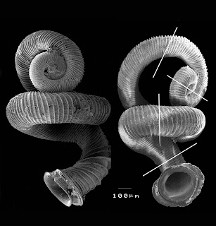
Vacation Post: Uncoiled!

Number 6...

...in the "Top 10 New Species of 2009"

Number 10 is pretty mind-boggling...
(continued...)

Update on problems with analysis

Ugh. Too much to blog about. The pace of computer work is totally different than with lab work (though in the end they seem equally labor-intensive), and I've made so many figures and gotten so many numbers in the past week, I barely know where to start...

Well, I guess I'll just blather about a couple problems I've been working through, but leave out all the charts and graphs and figures for the time being:

500-fold sequence coverage still "misses" parts of the genome:

We got a ton of data. For our controls, it was surely massive overkill. Nevertheless, "read depth" (how many read mappings cover a particular position) still varies by a substantial amount. There are numerous sources of this variation (%GC being one that is quite apparent), but I am most worried about variation in "read depth" due to the alignment algorithm I'm using to map reads to the genome.

As I try to root out artifacts in my discovery of putative recombination-associated mutations, I confront the fact that "read depth" is on average reduced when recombinant donor segments are mapped back to the recipient genome, so the novel mutations I found in these strains are on average supported by far fewer sequence reads than the average base... Most of them still look pretty solid to me (though there are several obvious artifacts), but I don't have a good rationale for whether or not to trust them.

I'm trying several things to work this out, namely by examinining the reciprocal mappings (using the donor chromosome as the reference).

So far, my analysis has a huge risk of false negatives:

Several problems here.

(a) Part of this problem and the last one is that I am using an alignment package that does not account for gaps (Maq). This means even a single nucleotide indel reduces "read depth" dramatically on either side (out to ~42 bases, or read length). See above.

(b) Another issue I'm facing with several of Maq's downstream outputs is that "read depth" is capped at 255. Presumably, they were conserving memory and only assigned a byte to this number. But what I haven't quite figured out is whether the SNP output (for example) is ignoring any possible SNPs where coverage exceeded 255. My cursory look at the more raw output (the "pileup") suggests this might well be the case. This could mean that I'm missing a lot, since the mean "read depth" per genome position in our datasets is ~500.

(c) Finally, I've been ignoring all Maq's self-SNP and "heterozygous" SNP calls in my downstream analysis using R. I presume that SNPs called in my mapping of the recipient genome to the complete recipient sequence are simply mutations between our wild-type Rd strain and the sequenced one. (As an aside, several hundred of the SNPs called by Maq were actually giving the correct base for an ambiguous base in the "complete" genome. I'd like to find a way to somehow revise the archived Rd sequence to get rid of all the ambiguous bases.) And I don't have a solid plan on how to deal with the "heterozygous" calls. Because the Maq assembly program can only have greater than or equal to two haplotypes, positions with mixed base signals are called heterozygotes. These is actually pretty cool and could reflect cool stuff like clonal variation, but largely these are probably due to multiply mapping reads and/or persistent sequencing errors.


Solutions: The solutions to these problems will initially largely be a matter of doing everything all again with different alignment software. My plan is to use the BWA aligner and SAMtools. BWA allows for gaps (so the "read depth" issue should be partially solved), and SAMtools not only keeps everything in a new agreed-upon standard format, but has several other tools, including what looks to be a better SNP caller (at least it has more modifiable settings). I would also like to try to do some de novo assembly, perhaps with Velvet, since we have such absurd coverage and a simple enough genome.

In the meantime, my R-fu has been improving, though I am convinced that I am missing some really basic principles that would make my code run a lot faster.
(continued...)

Mutagenic recombination?

Okay, this is pretty cool. I will probably discover that it’s just some artifact of the mapping, but digging into the transformant data some more reveals what appears to be a high number of mutations within recombined segments (alleles that have neither donor nor recipient identity)...

For this analysis, I used much more stringent criteria for calling SNPs, so that low quality SNP calls would not contaminate the result. This is particularly important here, since we might expect to get lower quality SNP calls in the recombinant segments, due to the relatively high divergence between the donor and recipient genomes and the limitations of current mapping algorithms.

For TfA, there were 802 unambiguous donor alleles and 19 high-quality novel alleles, while for TfB, there were 902 unambiguous donor alleles and 21 high-quality novel alleles.

The two plots below indicate the presence of unambiguous donor alleles in blue bars going to 1 (which defined the recombinant segments), and the presence of unambiguous mutant alleles in red bars going to -1. (Click to enlarge)

That looks pretty striking! Mutations are clearly clustered into the recombined segments!

A few of the "novel alleles" in the two genomes are shared. 4 of 6 are in the first overlapping donor segment, and the other two are outside the donor segments. It is still early to be too confident in this result, but still! It is very suggestive.

I’ve never really taken the supposed causal connection between recombination and mutation too seriously, since the evidence mostly seems correlative to me, but if this result holds up, I think it will be a uniquely clear-cut example of mutations induced by recombination.

Before being confident in the result, I need to map the data back to the donor genome, and cross-check the result. If that works, some simple PCR and traditional sequencing should readily confirm or refute this deep sequencing result. (continued...)