Showing posts with label computers. Show all posts

Friday, November 6, 2009

Weening myself off of Excel

In some sense, the computing I did today isn’t really useful, since I already worked out these things using Microsoft Excel. But I’ve been ordered by my bioinformatics consultants to stop with the Excel already. So as practice, I worked out some of the expected features of degenerate oligos again, but this time using R.

The main motivation for doing this besides practice is that I am fairly sure we should be ordering degenerate oligos with more degeneracy than we have previously considered. I won't make that argument here, but just repeat some analytical graphs I'd previously made.

It took a while (since I’m learning), but was still much more straight-forward than doing it in a spreadsheet. The exercise was extremely useful, as I learned a bunch of stuff (especially about plots in R), while doing the following:

Problem #1: Given a percentage of degeneracy per base, d, in an n length oligo, what is the proportion of oligos with k mismatches?
Answer #1: Use the binomial distribution. For a 32mer with different levels of degeneracy (shown in legend):
Problem #2: Given a million instances of such an oligo, how well would each possible oligo with k mismatches be observed?
Answer #2: Simply adjust each of the above values by dividing the number of classes within each of k mismatches (i.e. choose(n, k)):
Problem #3: If some number of bases, m, in the n-length oligo are “important”, what proportion of oligos with k mismatches will have x “hits”?
Answer #3: Use the hypergeometric distribution. The below plot is as for Problem #1 for 0.12 degeneracy, but with the # of hits broken down for each k:
I didn't try super-hard to make the perfect graphs, but it did take some effort to make a stacked bar plot...
(continued...)

Tuesday, October 27, 2009

Sets of Snps

So I’ve got pure DNA from my transformants, pretty much ready to send off for our first Illumina runs. I’m just doing a few simple checks with PCR and digestion to make sure everything is kosher.

But there is this little fear in my head about what I’ll do when I get the massive datasets. I got a hold of some example Illumina GA2 paired-end data taken from E. coli K12. Since I don’t have any data of my own yet from H. influenzae, this seemed like a good dataset to start learning how to do the initial data analysis.

I decided to go with the most widely-used reference-mapping software, called “Maq” for “Mapping and Alignment with Quality”. I can see why it’s widely-used; it is a breeze to install and use, which is the primary requirement for end-users to like a given piece of software. I’ve started dealing with just single-end reads from only one lane. The data is several years old, so there are “only” a few million reads of 35 base-pairs. Nevertheless, this represents nearly 20X sequence coverage of the E. coli K12 genome.

I’ll keep the Maq overview brief, since I went through it in lab meeting and Maq’s documentation is largely quite good (with the caveat that there are some challenges interpreting the meaning of all the columns in the different outputs). In short, Maq takes a “FastQ” file (which is the sequence data, including quality scores) and a “FastA” file (the sequence reference), converts them into a binary format (which is apparently helpful for making the mapping algorithm fast), and then maps individual reads to the reference, allowing up to 2 mismatches. The “pile-up” at each position is used to decide the “consensus base” at that position, based on the majority base and associated quality scores. The mappings can be extracted from the binary output using additional commands.

Here, I’ll focus on the .snps output (obtained by cns2snp... from the man page), since this will be the most straight-forward way for us to define recombinant segments in our transformants. I’m keeping things simple still, so there are a lot of other issues I could get tangled up in, other than the ones I’ll discuss here.

So I “Maqed” this one FastQ dataset from E. coli K12 (I’m calling it s11) against two different reference sequences:
  • K12 -> NC_000913.fna
  • O57 -> NC_002695.fna
The first is a sort of control for how the consensus base caller is working. Since the sequencing is from K12 DNA, most consensus bases called by Maq should match the reference. Occasionally some “SNPs” might appear. These could have several sources:
  1. Spurious due to low coverage and high error
  2. Actual mutations between the original completely sequenced K12 and the K12 used for the Illumina sequencing
  3. Clonal variation where the consensus-calling favors the variant sequence.
The second is to call SNPs between the two strains. I would expect that the number of SNPs called against O57 would vastly exceed that of K12.

This is easily decided with a little UNIX command on the two files to count the lines (which each correspond to a SNP call):
> wc -l K12s11.snp O57s11.snp
6051 K12s11.snp
64217 O57s11.snp
Indeed, there are 10X more SNPs running s11 against O57 than against K12. The several thousand SNPs called against K12 are likely mostly errors. Maq doesn’t always assign the consensus base with A, C, G, or T, but with any of the other IUPAC nucleotide codes, so many of these “SNPs” are probably quite low confidence.

That’s all fine and good, but now what? How can I tell how well this s11 dataset did at calling all the SNPs between K12 and O57? I resorted to using Mummer’s Dnadiff program (previously discussed here) to compare the two reference sequences to each other and extract the SNPs. If the s11 dataset really did a good job sequencing the E. coli genome, there should be a strong overlap between the SNPs called by Mummer and those called by Maq.

(Here’s a GenomeMatcher DotPlot run with Mummer)
Again, UNIX came to the rescue, thanks to this page I found that provides UNIX commands for working with “sets”.

First, I had to get the appropriate three columns from the two SNP files:
  1. the reference genome position (in O57)
  2. the reference base (also from O57)
  3. the query base (the SNP in K12; the consensus base call for Maq or the SNP call for Mummer).
Here's how I made those files:
> cut -f 2 -f 3 -f 4 O57s11.snp > maqSnp.txt
> cut -f 1 -f 2 -f 3 O57vsK12.snps > mumSnp.txt
This provided me with my two sets, one called maqSnp.txt and the other mumSnp.txt. Here’s their lengths:
> wc -l maqSnp.txt mumSnp.txt
64217 maqSnp.txt
76111 mumSnp.txt
Notably, Mummer called many more SNPs than Maq. I think this is largely because the SNP output from Mummer includes single-nucleotide indels, which Maq misses since is does an ungapped alignment. I’m not sure how to deal with this, but in our real experiments, they should still be discoverable, since we’ll map our reads to both donor and recipient genomes. Also, there are numerous “SNPs” in the Maq file that are non-A, C, G, T consensus bases, which will largely be absent from the Mummer comparison.

So, then it was a piece-of-cake to count the SNPs in the intersection of the two sets. Indeed there were several ways to do it, my favorite of which was:
> grep -xF -f maqSnp.txt mumSnp.txt | wc -l
57179
So:


That’s a whole lotta overlap! Happy! When I get the real transformant data, this will help me tremendously.

(continued...)

Thursday, October 15, 2009

Computing Bootcamp

Whew, I’ve really fallen behind on my blogging... Last week, a good friend of mine came into town for a “northern retreat”, in which he hoped to get work done on a paper. Instead, he and I drank enormous amounts of beer and did an enormous amount of computing with the Haemophilus infuenzae genome (at least by my standards). While the beer probably didn’t help anything, the computing did.

I’ll go over some of what we did in future posts, but right here I just want to outline some of the computing lessons I learned looking over his shoulder over the week. Many of these lessons have been given to me before and are likely quite basic for the real computationalists out there, but somehow I’ve emerged from the computing emersion with a lot more competence and confidence than I had before...


Here's three useful things I'm getting better at:

(1) Avoid using the mouse. The more that can be accomplished from the command line and using keystrokes, the better. From the command line, tab-completion and cursor-control of the command history make issuing commands far more efficient. The coolest keystroke I’ve now picked up the habit of in the Mac Leopard OS is Cmd-Tab, which takes you to the last active open application (and repeated Cmd-Tabs cycle through the open applications in order of their previous usage). This is perfect for toggling between the command-line and a text-editor where one can keep track of what one is doing.

(2) Toggle between the command-line and a text-editor constantly. Rather than trying to write a whole script and then run it from the command-line, it was far easier and faster to simply try commands out, sending them to the standard output, and cobble together the script line-by-line, adding the working commands to a text document. This has three useful effects: (1) Bugs get worked out before they even go into a script, (2) It forces one to document one’s work, as in a lab notebook. This also ended up being quite useful for my lab meeting this week, in which I decided to illustrate some stuff directly from the terminal. (3) It is forcing me to work “properly”, that is sticking with UNIX commands as much as possible.

(3) Learn how the computer is indexing your data. This point is probably the most important, but also the one that is taking me the most effort. I’ll illustrate with an example (which I’ll get into in more scientific detail later):

The output of one of our scripts was a giant 3 column X 1.8 million row table. I wanted to look at a subset of this huge table, in which the values in some of the cells exceeded some threshold. At first I was doing this (in R) by writing fairly complicated loops, which would go through each line in the file, see if any cells fit my criteria, and then return a new file that only including those rows I was interested in. When I’d run the loop, it would take several minutes for finish. And writing the loop was somewhat cumbersome.

But the extremely valuable thing I learned was that R already had all the data in RAM indexed in a very specific way. Built-in functions (which are extremely fast) allowed me to access a subset of the data using a single simple line of code. Not only did this work dramatically faster, but was much more intuitive to write down. Furthermore, it made it possible for me to index the large dataset in several different ways and instantly call up whichever subset I wanted to plot or whatnot. I ended up with a much leaner and straightforward way of analyzing the giant table and I didn’t need to make a bunch of intermediary files or keep track of as many variables.

Next time, I’ll try and flesh out some of the details what I was doing...
(continued...)

Wednesday, September 30, 2009

Struggling with the Background

Previously, I had shown some preliminary analysis of Rosie’s simulated uptake data of chromosomal DNA fragments. Rosie also sent me simulated uptake data of degenerate USS sequences (using a 12% degeneracy per position in this USS consensus sequence :

5’-AAAGTGCGGTCAAATTTCAGTCAATTTTT-3’).

So what can I do with this dataset? Well, first, since Rosie also provided me with the “scores” for each sequence, I could plot a histogram of the scores for the 100 selected and 100 unselected sequences, showing that the uptake algorithm seems to work pretty well.

Here's the histogram:
Notably, even the unselected sequences have rather high scores, when compared to the same analysis of genomic DNA fragments. This is unsurprising, since the sequences under selection in this degenerate USS simulation are all rather close to the consensus USS.

Here’s the histogram from the genomic uptake simulation again (just to compare):
(I think the reason for the difference in the “selected” distributions is due to a different level of stringency when Rosie produced the two simulated datasets.)

That’s all fine and good, but now what? With the genomic dataset, I could use the UCSC genome browser to plot the location of all the fragments I was sent, but this consists of two alignment blocks of sequence that look markedly similar.

The obvious thing to do was to make Weblogos of the two different datasets… The unselected set should have very little information in it, while the selected set should contain information. In doing this, I discovered a rather important issue… The on-line version of Weblogo does NOT, I repeat, does NOT account for the background distribution.

This is a problem. It means that whenever you make a Weblogo (on the webserver) from your alignment block, it is assuming that each base is equally likely to occur at a random position. This is why the y-axis in all Weblogos plots always has a maximum of 2 bits when using DNA sequence. Why is this a problem? First of all, if one is using an AT-rich genome, as we are, then the information content of any G or C is underestimated and any A or T is overestimated.

So how does Weblogo calculate the information content of each position in an alignment block? From the Weblogo paper (link found at the Weblogo website):
Rseq = the information at a particular position in the alignment
Smax = the maximum possible entropy
Sobs = the entropy of the observed distribution of symbols (bases)
N = the number of distinct symbols (4 for DNA)
pn = the observed frequency of symbol n

The log2 is there to put everything in terms of bits.

So for DNA (4 bases), the maximum entropy at a position is 2 bits. Makes perfect sense: 2 bits a base. However, this only makes sense if each base is equally probable for a randomly drawn sequence. Now for purposes of gaining an intuition for different motifs, this isn’t really a big deal, although it does complicate comparing motifs between genomes.

When this isn’t the case (probably much of the time), then different measures have been used, namely the “relative entropy” of a position. This is an odds ratio of the observed probability and the background probability. Apparently, the off-line version of Weblogo can account for non-uniform base composition, but I haven’t tried installing it yet, nor any other software out there that handles variation in GC content.

Why? Because what we need for our degenerate sequences is a different background distribution at each position! So, the first position in the core is 88% A, but the third position is 88% G!

To illustrate the problem, here is a Weblogo of the selected set:
Here’s the unselected set:
Looking closely, it is clear that there are differences in the amount of “information” at each position. So in the strong consensus positions of the USS, the selected set has higher “information” than the unselected set, while at weak consensus positions, that’s less true.

But the scaling of each base here is completely wrong. There isn’t nearly a bit of information at the first position in the unselected set. We expected 88% A. The fact that there are mostly As in the alignment block at the first position is NOT informative. In fact, if all was well, we’d get zero bits at all the unselected positions!

What to do? I tried to make my own logo, using the known true background distribution at each position. I won’t belabor the details too much at the moment, except to say that I had to figure out what a “pseudocount” was and how to incorporate it into the weight matrix, so as to not ever take the logarithm of zero.

Here’s the selected set of 100 sequences:
Here’s the unselected set of 100 sequences:
(Note that I somehow lost the first position when I did this, so the motif starts at the first position of the core.)

This actually looks quite a bit better, or at least more sensible. A few things worth noting:
  • I think if we did thousands of unselected sequences, we’d pretty much get zero information from that alignment, which is what we would want, since that’s just the background distribution.
  • Some values are negative. This is expected. Since these are scaled to log-odds ratios, when the frequency of seeing a certain base is less than the expected background frequency, a negative number emerges.
  • The scale is extremely reduced. Every position is worth less than 0.3 bits. This is also expected. One description I’ve seen about how information content can be thought about is how “surprised” one should be when making an observation (there’s even a unit of measure called a “suprisal”!). Since we are drawing from an extremely non-uniform distribution that actually favors the base that’s expected to be taken up by cells better, we are basically squashing our surprise way down. That is, getting an A at the first position of the core is highly favored, but it’s the most likely base to get anyways, even in the absence of selection.
  • The unimportant bases in the USS have the most information content in the selected set. At first this bothered me, but then I realized it was utterly expected for the same reason as above. For example, at position #18 above (sorry, it’s position 19 in the Weblogos), the selection algorithm doesn’t really care what base is there. That means that the selected set will let mutations at that position (from A to something else) come through, which will be surprising, when compared to the background distribution!
(ADDED LATER: Actually, this last point is wrong. The reason for so much information at the weak positions is related to the matrix that was used to select the sequences, not from surprise. I'll try and get a proper dataset later and redo this analysis. To some extent, the positions will still have some information, as partially explained in my erroneous explanation above, but not nearly so much.)

Whew! I’ve gotta quit now. There’s a lot more to think about here.
(continued...)

Friday, September 25, 2009

More simulated uptake

Thanks to Rosie eliminating the int function from her Perl model, I got to take a look at some more simulated uptake data. Last time, there were several issues, which now seem solved. This time to model uptake, she used the real genomic USS position weight matrix to stochastically select 500 bp fragments from the first 50 kb of the Haemophilus genome. I got 200 from the forward strand and 200 from the reverse complement strand, along with a set of random fragments. This is 4X spanning coverage of the 50 kb…

Below is the way the data looked in the UCSC genome browser, added as custom tracks (click on the figures to enlarge).
From the top, the tracks are:
(1) Chromosome position
(2) 400 random fragments (shades of brown).
(3) 400 selected fragments (shades of blue).
(4) Positions of “perfect core” USS motifs (5’AAGTGCGGT-3’) on either strand
(5) RefSeq gene annotations.

Here’s a bit of the 50 kb zoomed in:
That looks pretty good for such low coverage! (In our real experiment, we expect to get several hundred times more data.) It’s starting to look like a real model of how uptake might look! The random fragments look roughly randomly distributed, and the selected fragments clearly show a punctate distribution around the “perfect core” USS sites.

Here’s a histogram of the scores of the best site on a given fragment for the random and selected datasets:
Indeed, the distributions are quite distinct, though notably the distribution of random fragments looks bimodal. This may simply be a feature of the genome, since there are so many USS sites… Worth thinking about though.

There are other details obscured in the browser figures: the shading indicates the relative score of the best site on the fragment (on a log scale), and each fragment also has orientation shown as a small arrowhead within the box. I’ve also associated each fragment with its score. So in the browser, I can easily check things out more carefully:
In this zoom, it’s clear that there is an excellent site to the left (just under 18,000), a weaker site to its right (~18,400; fragments are overlapping with the left-most site; no perfect core), and a pair of sites on different strands with different scores to the right (~19250). I can also retrieve the sequence associated with a given fragment to see if I can spot the USS site within it. And if I really zoom in, the DNA sequence is listed at the top.

It’s not really so easy to see what’s going on with all these overlapping fragments, so my next task will be to convert this data from fragment positions to spanning coverage per chromosomal position (though I’ll probably bin positions, perhaps every 100 bp to keep things reasonably small for now). I will take a stab at doing this properly (with a script) but may wimp out and do it in Excel. If I can then muscle this data into a WIG formatted file, then I’ll be able to plot the data in a way where “good” sites will look like peaks in coverage…
(continued...)

Tuesday, June 9, 2009

Supragenomicisticexpialidocious


Howzabout that “supragenome”?

Polymorphic gene content

Genome sequencing efforts have captured substantial variation in the gene content among closely related bacteria. For example, this nice study by Hogg et al. 2007 compared the genome sequences of thirteen Haemophilus influenzae: They found a “core genome” of ~1500 genes, along with another accessory (or contingency) genome of ~1300 genes. Any given isolate had a subset of the accessory genome, numbering around a few hundred extra genes beyond the core in each isolate.

So any two isolates have substantial amounts of DNA that is unshared. For example, Hogg et al. report that the Kw20/Rd and 86-028NP isolates differ by nearly 400,000 bp within only ~250 indels (Table 5-- mean size: ~1.5 kb, median size: ~300 bp). The genomes are < 2 Megabases long, so that’s about 20% of these chromosomes that is non-homologous.


(As an aside, the Hogg et al. paper’s methods section introduced me to MUMmer, which I previously discussed. The indels and other rearrangments are essentially defined by breaks in the alignment produced by the nucmer utility. More on this in the future...)

There are several possible arguments related to uptake specificity and the "supragenome":


Uptake specificity for variation?


Large variation in orthologous gene content suggests to Hogg et al. and others a “distributed genome hypothesis”, in which natural transformation can shuffle (or re-assort, or segregate) the accessory genes between isolates. This would then presumably allow for the rapid acquisition and loss of different genes (diversification) from within a given genetic background and thus perhaps rapid adaptation to environmental changes (or shifting host defenses). The “distributed genome hypothesis” is then implicitly related to the “sex hypothesis” for the maintenance of natural competence.

Uptake specificity for conservation?

On the other hand, natural transformation could also maintain the “core genome”. Thus, if there is plenty of conspecific DNA uptake, any bit of “core genome” taken up could be replaced in a cell that had lost it. This nice study by Treangen et al. 2008 using several neisserial genome sequences showed that DNA uptake sequences (DUS, the neisserial equivalent of USS) existed at a higher density in “core” regions of the genome than in the substantial alignment gaps between isolates (containing indel poymorphism).

Again, there is some indication of the “sex hypothesis” for the maintenance of natural competence, but it works in the opposite direction, maintaining the core rather than shuffling the accessory. I think the argument goes like this: (1) The core genome likely defines the more essential portions of the genome, since by definition any accessory genes are not required to live. (2) DUS could have been selected for within this partition of the genome, since it would help to maintain the more essential gene functions within a population. (3) Therefore the high number of DUS sequences could be a product of natural selection to maintain the integrity of the “core genome”.

Uptake specificity for no reason in particular?

However, there’s another possibility the authors partially explore that does not involve selection for DUS distributed throughout the genome, but represents almost the opposite model. Instead of selection, pehaps DUS accumulate due to happenstance intrinsic biases in the uptake and/or recombination machinery by a neutral molecular drive. So sequence variants that arise with a higher chance of being taken up later are more likely to spread through populations than variants with a lower chance of uptake. Thus the “core genome” could partially be that way, i.e. conserved across isolates--not exclusively because of essentiality or usefulness--but also by virtue of containing lots of DUS. So rather than DUS being selected for in order to maintain the core genome, segments of DNA containing DUS are simply mre easily replaced in lineages that lost them.

An affiliated idea suggests that if some accessory genes were from distant relatives and arrived by horizontal transfer by some mechanism besides natural competence, these sequences would not have had time to accumulate uptake sequences yet. Thus the paucity of DUS in the accessory genome might be in part due to the more recent arrival of that sequence in the genome, so the effects of drive have not yet become evident, rather than a specific selection pressure to maintain DUS in more important segments of the genome.

(The Treangen et al. paper introduced me to another genome alignment tool called M-GCAT. I’ve played with it a bit and managed to produce some figures effectively the same as what appears in their supplementary data-- the picture above (along with alignment files resembling multi-FASTA format) but have the unfortunate problem of being unable to re-load analyses I’ve performed later due to some kind of Python error. More in this later as well...)

How to analyze the core and accessory genomes myself?

I’ve clearly got a lot more thinking to do regarding these core and accessory genomes... Especially in light of the horizontal gene transfer issue.

But first I’d better figure out simply how to define the core and accessory genomes more specifically.

I’ve begun this by examining the gaps in the .rdiff and .qdiff output of dnadiff (a pairwise comparison of two genomes) to try and do some basic analysis myself. In a future post, I’ll report on my progress with this, but for now, I’ll just mention that most of the gaps are not strictly insertions or deletions, but are rather insertional deletions. Alignment gaps include both reference and query bases. But I still need to try and understand how dnadiff produced its .report output before I can get much further...
(continued...)

Wednesday, June 3, 2009

There's a lesson here somewhere

A recent email exchange with a local computer expert, explaining one reason I normally avoid directly seeking help until I really need it (this also applies to statisticians):
Me (paraphrased): Er... help... with things...
Me (a little later): It worked like a charm! Soon after I asked you for help, I worked it out... Figures.
Local Expert (soon thereafter): Glad to be of service!
Nevertheless this method is tried and true! Thanks, Alistair!

Here's another tool I recently checked out...

CGView made a rather nice figure for default settings: (from out to in) genes, %GC base composition, GC skew. There seems to be several other ways to further configure the file. In particular, I was interested in the plot of GC skew. Changes in sign (between purple and green) can indicate origins and termini of replication, due to mutation rate differences between the leading and lagging strands of replication. It's not immediately obvious what position should be the starting coordinate for a particular genome, but for PittEE, I suppose I'd guess the origin as the hour hand a little before 6:30...


Details on how I made that:
I didn't have too many issues running the package. It needed a bit of BioPerl (Bio::SeqIO) to interpret the GenBank file, which I knew I'd downloaded in my GBrowse installation quest, but for some reason, I needed to specify the correct Perl sublibrary to a variable called $PERL5LIB.
> export PERL5LIB=$PERL5LIB:/sw/lib/perl5/5.8.6/

I still have a lot more to learn about working at the command line, since each time I start a new terminal, I need run this command again, if I want to use CGView.

After that, I went to the directory containing the GenBank file for one of the complete genomes (86-028NP.gbk), and typed:
> perl /path/cgview/cgview_xml_builder/cgview_xml_builder.pl -sequence PittEE.gbk -size small -output PittEE.xml
(/path defines is the place I put the CGView directory that downloaded. Mine was in a directory /path = /Users/my_name/bin)

This converted the GenBank file into an XML file suitable for reading by cgview.jar. Pretty cool! (I didn't have to think about JAVA being there, since it was already installed.)

Then invoking java:
> java -jar /path/cgview/cgview.jar -i PittEE.xml -o PittEE-map.png -f png
Presto! The figure above.
(continued...)

Friday, May 29, 2009

Enumerating their differences


I took a break from working on GBrowse today to try and do some genome-wide alignments of the sequenced Haemophilus influenzae isolates, and it's gone remarkably smoothly. The more I play around with the command-line, the more I'm finding it an excellent and efficient way to compute. Still hurts my head after a while.

I went to GenBank and downloaded FASTA and GenBank files for the four completely sequenced strains: our reference KW20-Rd and three clinical isolates found in ear infections...

I first used a program called MAUVE, recommended by my predecessor postdoc, which produced the lovely looking colorful plot above, comparing KW20-Rd and 86-028NP. It was extremely easy to use (though I only tried default settings). The only thing I had to do was change the GenBank file extensions from .gb to .gbk and everything worked great.

The colored blocks indicate syntenic regions and the relative sequence similarity within a block is indicated on the y-axis. When a block is in an inverted orientation, it falls below the line. When there's white-space, that's indicating a large insertion absent from the other strain. I can sort of piece together the rearrangements separating the two strains by eye, but even easier is a button in the MAUVE window that took me to a GRIMM analysis page that simply gave me a minimal path of inversions between the sequences. Sweet! It counts six big inversions (some overlapping) to give the rearrangements needed to get from KW20-Rd to 86-028NP.

My next task was to try and actually enumerate the differences between the strains. MAUVE makes a pretty picture (and also has a nice browser-like visual annotation based on the GenBank file), but I'd also simply like to count all the SNPs, indels, and other rearrangment breakpoints between the strains. I couldn't figure out how to do this in MAUVE and didn't feel like trying to parse its alignment file.

So I got an altogether different genome-wide alignment suite of programs called MUMmer. At first, I was scared of it, since it involved command-line arguments, and I'm sort of fried on that for the week. But after installing and compiling the suite of programs, I found it incredibly easy to use. For this I used FASTA files, and invoked the dnadiff program, which uses a bunch of the MUMmer utilities for pairwise comparisons. It did each pairwise analysis in under 10 seconds, providing me with a series of different output files. I was impressed.

I spent most of the day learning what these files contained and playing with the settings, and it's pretty much got everything there I want, as long as I can parse the files correctly. I decided to start with the SNPs between the reference KW20-Rd genome and the other three. There as one little glitch in the nice .report output file, in which it didn't call all classes of SNPs (it was excluding G-T differences from the report), so I dug into the code and successfully altered it to give the full list. Here's what I found:
There's >40K SNPs between the reference and each of these others. As would be expected, the transition/transversion ratios are ~2. The number of SNPs going from X->Y and Y->X were effectively identical for all comparisons, so I added them together in the above plot. It also looks like toggling between G and C is a particularly difficult transversion for some reason. Anyways, piles of SNPs, as expected.

For my next trick, I'll look at the distribution of indel and rearrangement polymorphism...
(continued...)

Thursday, May 28, 2009

GBrowse Update (boring, except the bit about the fish)

I finally succeeded in my attempt to put a functioning GBrowse installation on my computer. My problem turned out to be extremely trivial and way upstream of the actual GBrowse installation. Now I’ve got to figure out how to correctly produce and configure a basic Haemophilus influenzae genome database...

My first big problem--now solved--was that I was unable to view webpages from localhost, that is I couldn’t view webpages served by Apache2 on my own computer. All kinds of other people have had such problems, but none of the help I found on forums seemed to help with my problem. Nevertheless, I did learn a lot more about the way that files are organized in Mac’s UNIX.

Luckily, in my forum perusal, I stumbled across a nice switch to the apachectl function, so that at the command line I could type: "sudo apachectl -t" or "sudo apachectl configtest". This gave me a syntax check of my Apache webserver configuration, which returned a convoluted syntax error. After checking the several files where the errors were called, I figured out that I’d failed to add a space between two separate statements in the configuration file I'd made that set my own permissions. Gah. Anyways, it works now. The problem WAS actually covered in several of the forums I'd searched (because Apple moved some things around in their latest Leopard upgrade), but that's no help when you type the needed file in wrong...

After that I had one additional problem, which was that I used all the default settings with the GBrowse install script, which put everything into the wrong or non-existent directories. When I repeated the install with the correct paths for Mac OS X 10.5.7 and Apache2, I suddenly had the Generic Genome Browser on my computer!

I found this site, which told me to redirect the installer to the following paths when prompted:
Apache conf directory? [/usr/local/apache/conf] /etc/apache2/
Apache htdocs directory? [/usr/local/apache/htdocs] /var/www/localhost/htdocs/
Apache cgibin directory? [/usr/local/apache/cgi-bin] /var/www/localhost/cgi-bin/
Presto! A working web server with a working genome browser!
I went to http://localhost/gbrowse/, and got a page annoucing:
Welcome to the Generic Genome Browser!
A happier moment of web surfing, I've not had since I found out about the fish with a transparent head.

Okay, nonetheless, I still haven’t gotten the Haemophilus influenzae KW20 genome properly working in the browser. I’ve gone through the tutorial pretty thoroughly and have correctly configured their tutorial Volvox database using a MySQL backend. It works fine.
My KW20 database seems to be correctly imported into MySQL, but nothing shows up on the webpage. I originally thought it had something to do with my configuration file, but now I suspect some kind of import defect. I’ve tried it two ways.

(1)Doing it in memory: Getting the GenBank file from NCBI, converting it with BioPerl’s conversion program, bp_genbank2gff3.pl, then loading it with BioPerl’s bp_bulk_load_gff.pl

(1) Doing it in MySQL with the GFF and FASTA files from TIGR’s homepage and using BioPerl’s MYSQL dumper, bp_seqfeature_load.pl (for which I can find no good link or man page).

Neither of these worked. I’ve been tweaking the configuration file and trying to reload the database in several ways. So far with no luck. But progress! I'm fairly certain I need to understand the Adaptors better...
(continued...)

Wednesday, May 13, 2009

Using a Computer


I’ve been working on installing the stripped-down open source genome browser, GBrowse, onto my computer. In order to do all this cool sequencing stuff I’m planning, I’ve got a lot of computer-learning curve to overcome. One thing that will be extremely useful both for learning and for our future plans will be to build my own Haemophilus influenzae genome browser.

So GBrowse installation looks pretty easy. But I do need to have various things installed (and configured properly) for it to work:

  • Apache (a webserver),
  • PHP (a webpage-writing scripting language),
  • MySQL (a database language),
  • Perl (a scripting language that’s useful for manipulating text),
  • Bio-Perl (a set of modular programs written in Perl),
  • and finally of course, GBrowse.
After that, I can add in my genome data in the form of GFF3 files and take it from there. (A BioPerl module will convert normal GenBank files into GFF3 files that the browser wants.) In the future, I hope to align the sequenced isolates into the browser, have some annotations, and eventually add custom tracks representing my sequencing runs.

Luckily all of these packages are open-source and freely available on the web. Unluckily, my skills on the UNIX command line are slow, and my ability to understand system files are apparently extremely limited.

I initially caused all sorts of havoc to my computer trying to get the basic Apache and PHP set-up working. If functioning properly, I should be able to serve my own webpages and see them in my browser. No such luck. After digging around in some forums, I found that many had similar problems, so started mucking around with sensitive system files as recommended on these forums.

This involved uncommenting out some lines of some seriously ugly looks configuration files used by Apache and making sure that I had permission to view my own webpages... I never made it work the way it was supposed to. I feel comfortable enough with text editors and the basic stuff on the command line, but I really don’t understand the hierarchy of the directories in UNIX. I’m sure that most of my problems are stemming from that.

Fortunately, I had actually been taking notes on everything I was doing to my computer! So I could back out and start over. I also discovered that some clever programmers had made things a lot easier for me by having back-ups of a lot of files around.For example the apache2.conf file that I’d tinkered with could simply be replaced by the apache2.conf.default that was sitting right there in the directory with it, so at the command line: cp apache2.conf.default apache2.conf

Next I discovered an easy way out: XAMPP, which was written specifically for the computer semi-literate to make all the configuring happen smoothly. I installed it, and Presto! Apache, PHP, and MySQL up and running with default localhost webpages appearing in my browser magically. WHEW!

Okay, so moving onto GBrowse... I already have Perl, and GBrowse has a handy install script that will get me BioPerl along with GBrowse itself. This ended up taking forever, because the CPAN mirror (which carries all the Perl stuff) kept kicking me off. Eventually, it all seemed to install, and I got a happy message:

########################################################
GBrowse is now installed. Read INSTALL for further setup instructions.
Go to http://localhost/gbrowse for the online tutorial and reference manual.
########################################################

But to NO AVAIL! The web address didn’t work, and I couldn’t find that INSTALL file for the life of me. (There’s a lot of files entitled INSTALL.) Criminy, I could already tell what happened, and more forum-searching, and more tinkering, it doesn’t matter because I still couldn’t fix it... Paths. My programs are looking for each other in the wrong locations.

XAMPP’s MySQL got broken, and Apache didn’t know where to look for GBrowse. I actually haven’t found it myself yet. So no dice. I need to figure out how to redirect the Paths, such that the XAMPP installation knows where GBrowse is sticking itself and XAMPP needs to know what happened to MySQL after installing BioPerl and GBrowse. Since I can’t tell those things myself, I guess I’m going to have to go back to the drawing board again...

Sigh... So close yet so far. But the note-taking has been utterly crucial. I, like Rosie, have always thought that I was doing “preliminary analysis” when using my computer for something other than Microsoft Office or Firefox, so always have to repeat work. But especially mucking around with my system files, I’m truly glad I kept track.

It may almost be time to wrassle up a real computer person to give me a hand...
(continued...)